Property-Driven Training

This chapter comes in two parts. The first asks what the standard machine-learning toolkit can do about the properties of Chapter 3: we train a network the ordinary way, put Chapter 3’s question to it, and then look at data augmentation and adversarial training, the two established methods for making a network more robust. The second part asks what is missing from that toolkit once the property we care about is an arbitrary logical specification rather than an -ball, and describes the property-driven framework that Vehicle is built to support. It closes with the experiment the whole chapter has been building towards: the network from the first part, trained for ten more epochs with the specification in its objective, and verified after every one of them.

Part I — Training for robustness with standard machine learning

Motivation

We begin with a question: how can we train a neural network to be more robust within a chosen ? Machine learning has a long tradition of methods for this, and two dominate. One re-trains the network on additional data drawn from inside the -balls around the training points; the other generates adversarial examples, the points inside each ball on which the network is closest to changing its answer, as training proceeds. We will look at both, after first seeing how robust a network trained in the ordinary way turns out to be.

Training with Loss Functions

Humans learn by making mistakes. The same is true of neural networks. Loss functions are a way of measuring the “magnitude” of a mistake made by a neural network. For a given training input, loss functions compute a penalty proportional to the difference between the output of the network and the true output (i.e., the training label). Formally, this is written as follows:

The function represents the network, whose optimisation parameters are , and and represent the sizes of the input and output tensors respectively.

One of the simplest (yet usable) loss functions is called mean squared error, defined as:

where is the total number of data points, is the label for data point , and is the model’s predicted value for . I.e., we find the difference between the prediction and the actual value, square it, and take the average across the training dataset.

The example later in this chapter classifies images rather than predicting a number, and for that the usual choice is cross-entropy loss. In the same notation:

where is the number of classes, which is also the size of the output tensor, is when data point belongs to class and otherwise, and is the probability the network assigns to class . Since only one term of the inner sum is non-zero, this is just the average of of the probability given to the correct class. The penalty therefore grows without bound as that probability approaches zero, which is what makes cross-entropy a better fit than mean squared error when the outputs are class probabilities rather than magnitudes.

One practical note: the networks we build below end in a plain linear layer, so they emit unnormalised scores rather than probabilities. Both PyTorch’s CrossEntropyLoss and TensorFlow’s SparseCategoricalCrossentropy apply the normalisation internally, which is why no softmax appears in the model definitions.

Models learn by iteratively tweaking their optimisation parameters with the goal of minimising the output of the loss function. The most common way to do this is using gradient descent. Formally, we wish to find the set of parameters that yields the least loss:

We are now ready to code all of this.

Getting Started with the Code

Let us start our first training pipeline. Recall that Chapter 3 ended with failing to verify robustness. We used the model that was already pre-trained. Let us now try to train a similar model from scratch, in the plainest way possible, and see how robust it turns out to be.

Here, we use the Fashion MNIST dataset to train a neural network. All files used in this example can be found in the chapter-4/chapter-code directory of the tutorial repository.

First, we need some data to train on. Nothing here is specific to Vehicle, and the same loader serves both the plain network we train in a moment and the property-driven one later in the chapter.

import torchvision
import torchvision.transforms as transforms
from torch.utils.data import DataLoader, Subset

BATCH_SIZE = 64
SUBSET_SIZE = 1024  # ensure SUBSET_SIZE mod BATCH_SIZE == 0

transform = transforms.Compose([
    transforms.ToTensor()
])

train_data = torchvision.datasets.FashionMNIST(
    root="./data", train=True, download=True, transform=transform
)
train_loader = DataLoader(
    Subset(train_data, range(SUBSET_SIZE)), batch_size=BATCH_SIZE, shuffle=True
)

import tensorflow as tf

BATCH_SIZE = 64
SUBSET_SIZE = 1024  # ensure SUBSET_SIZE mod BATCH_SIZE == 0

(train_images, train_labels), _ = tf.keras.datasets.fashion_mnist.load_data()

train_images = train_images[:SUBSET_SIZE].astype("float32") / 255.0
train_images = train_images[..., None]  # add channel dim -> (N, 28, 28, 1)
train_labels = train_labels[:SUBSET_SIZE].astype("int32")

train_loader = (
    tf.data.Dataset.from_tensor_slices((train_images, train_labels))
    .shuffle(SUBSET_SIZE)
    .batch(BATCH_SIZE)
)

Three of these choices are worth explaining.

SUBSET_SIZE restricts training to the first 1024 images. Plain training would happily run over all 60,000, but evaluating a robustness property is far more expensive, so a subset keeps the second half of this chapter runnable while still showing the effect. Keep it an exact multiple of BATCH_SIZE; the reason becomes clear later, when we pass n=BATCH_SIZE to the constraint loss.

There is deliberately no normalisation step. ToTensor (and dividing by 255 in TensorFlow) leaves pixel values in , and that is where we leave them. This is worth dwelling on, because the usual recipe for image classifiers subtracts the dataset mean and divides by its standard deviation, and doing so here would quietly break the chapter.

The reason is that our specification says what a valid input is: validImage x = forall i j . 0 <= x ! i ! j <= 1, and the .idx datasets we hand to the verifier hold pixels in exactly that range. Normalising during training would move the network’s input space to roughly while leaving the verifier’s input space at — so the network would be verified on inputs unlike any it was trained on. Worse, would silently denote two different regions: a perturbation of in normalised units is only of a raw pixel, so training would enforce a neighbourhood almost three times tighter than the one being checked.

Keeping the data in the range the specification talks about costs us nothing here — the network below trains perfectly well on raw pixels — and it keeps a single meaning for across training and verification. Part II returns to this: it is a small instance of the general difficulty of interfacing a logical specification with an optimisation objective. One of the exercises in this chapter will give you a chance to reconstruct the whole training-verification pipeline with normalisation baked into the training.

Finally, note that the two frameworks store images differently: PyTorch’s ToTensor produces channel-first batches of shape (N, 1, 28, 28), whereas here we append the channel dimension last for TensorFlow, giving (N, 28, 28, 1). It makes no difference to the network we are about to train, whose first layer flattens its input either way, but it will matter once we start handing images to a specification.

Training the network the ordinary way

With the data in place, the rest is unremarkable supervised training. The architecture is small — two hidden layers — which is deliberate: a simpler network has smoother decision boundaries, and is therefore easier both to train and to verify.

import torch
import torch.nn as nn

model = nn.Sequential(
    nn.Flatten(),
    nn.Linear(784, 64),
    nn.ReLU(),
    nn.Linear(64, 32),
    nn.ReLU(),
    nn.Linear(32, 10)
)

optimizer = torch.optim.Adam(model.parameters(), lr=1e-3)
cross_entropy = nn.CrossEntropyLoss()

num_epochs = 150  # the script ships with 5; the table below uses 75, 100 and 150

for epoch in range(num_epochs):
    running_loss, correct, seen = 0.0, 0, 0

    for images, labels in train_loader:
        optimizer.zero_grad()
        logits = model(images)
        loss = cross_entropy(logits, labels)
        loss.backward()
        optimizer.step()

        running_loss += loss.item() * labels.numel()
        correct += (logits.argmax(1) == labels).sum().item()
        seen += labels.numel()

    print(f"Epoch: {epoch + 1}, mean loss: {running_loss / seen:.4f}, "
          f"train accuracy: {100 * correct / seen:.1f}%")

Nothing in that objective mentions robustness. The only thing being minimised is cross-entropy, exactly as in any introductory classification example. This is the complete script vanilla_classifier.py in the chapter code.

To verify the result we need it in ONNX form:

model.eval()
torch.onnx.export(
    model,
    torch.randn(1, 1, 28, 28),
    "vanilla-experiment/onnx_models/vanilla_classifier.onnx",
    input_names=["input"],
    output_names=["output"],
    external_data=False,  # required for Marabou verification
)

Asking Chapter 3’s question of our own network

We now put this network to exactly the question Chapter 3 asked: the same specification, the same , the same fifty images.

vehicle verify \
  --specification fashionRobustness-solution.vcl \
  --network classifier:vanilla_classifier.onnx \
  --parameter epsilon:0.005 \
  --dataset trainingImages:0-49Images.idx \
  --dataset trainingLabels:0-49Labels.idx \
  --solver Marabou

On 1024 images this network reaches 98% training accuracy by about epoch 75, and 99.9% by epoch 150. Training it well past the point where the task has essentially been learned gives:

The first three columns are measured during training, on the 1024 images the network learns from. The last three are measured afterwards by Vehicle, on the fifty images of Chapter 3’s set — which are test images, held out of training. So correctly classified reports generalisation rather than memorisation, and it is a different quantity from the training accuracy beside it.

Reading down the training columns, the mean loss almost halves between epochs 75 and 100 and falls by a factor of seven and a half by epoch 150. Reading down correctly classified over the same span: 38, then 38, then 37. All that extra optimisation bought no improvement in generalisation whatsoever.

The two robustness columns have to be read against correctly classified, not against 50. An image the network already gets wrong cannot be robust, because advises perturbedImage label fails at zero perturbation; such an image is counted as a failure for a reason that has nothing to do with robustness. So correctly classified is a ceiling on how many images could possibly be proved robust.

At the network sits exactly one image below that ceiling at every checkpoint — 37 of 38, 37 of 38, 36 of 37. The apparent dip at epoch 150 is the ceiling moving rather than robustness changing: one image left the correctly classified column and took its robustness result with it.

The column tells a more interesting story. Here the checkpoints do not agree, and they disagree in an orderly way: 25 provable images at 75 epochs, 22 at 100, 21 at 150. Training for longer has made the network less robust, and steadily so.

Note that this is not the ceiling moving. Over those same checkpoints the number of correctly classified images goes 38, 38, 37 — down by one — while the number proved robust falls by four.

This is what one would expect. Once the training data is fitted, further optimisation of cross-entropy cannot change which side of the decision boundary the training points fall on, so it draws the boundary closer to them instead, buying greater confidence on answers that were already correct. The margin around each point narrows. A neighbourhood of radius is too small to notice; one of radius is not. So robustness is not just a quantity the task objective fails to measure. It is one the task objective erodes, and the erosion only shows at a radius wide enough to see it (Madry et al., 2017) Madry, A., Makelov, A., Schmidt, L., Tsipras, D., & Vladu, A. (2017). Towards deep learning models resistant to adversarial attacks. arXiv Preprint arXiv:1706.06083. . If we want robustness, it has to appear in the objective itself.

How much room is there to improve? Before turning to methods, it is worth asking how much of a robustness problem there is to solve, and that depends on . The figures above mix two effects together, because thirteen of the fifty images are misclassified and so fail at zero perturbation. Setting those aside and keeping only the 37 images the epoch-150 network classifies correctly, the same specification at two radii gives:

Same network, same images; only the size of the neighbourhood differs. A four-fold increase in the radius turns one failure into sixteen, so the near perfect robustness at was less a property of the network than of the question we asked it: the neighbourhoods were small enough that almost nothing could go wrong inside them.

This sets the terms for the rest of the chapter. To ask whether adding robustness to the training objective helps, we need a radius at which the network is genuinely vulnerable. At there is one image to win back; at there are sixteen.

We will first consider traditional machine learning methods that were introduced to address the problem of adversarial robustness.

Data augmentation

Both established methods train on extra inputs drawn from around each data point; they differ in how those inputs are chosen.

Data augmentation generates additional training data inside the -ball of each original point, by rotating, cropping, flipping or randomly perturbing it, and gives every new point the label of the point it came from. Training then proceeds as usual on the enlarged data set, in the hope of improving the network’s average-case robustness (Shorten & Khoshgoftaar, 2019) Shorten, C., & Khoshgoftaar, T. M. (2019). A survey on image data augmentation for deep learning. J. Big Data, 6(60). .

The method has two problems, both to do with labels. If an original point lies close to the decision boundary, an augmented point may fall on the other side of it while still inside the ball, and so carry the wrong label:

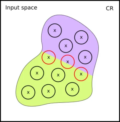
And if the balls of two points on opposite sides of the boundary overlap, the same location in input space can be generated twice, once with each label:

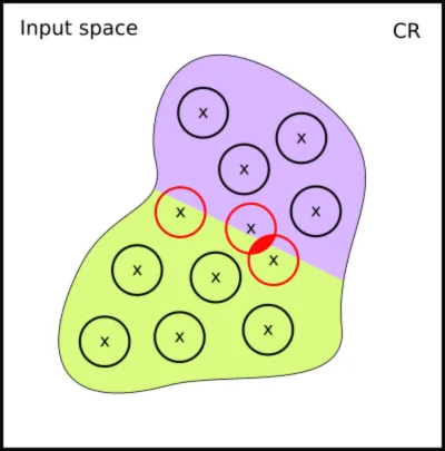
Training on data with these inconsistencies does not reliably make a network robust, so the method is not viable for the kind of robustness we want to verify.

Adversarial training

Adversarial training (Madry et al., 2017) Madry, A., Makelov, A., Schmidt, L., Tsipras, D., & Vladu, A. (2017). Towards deep learning models resistant to adversarial attacks. arXiv Preprint arXiv:1706.06083. also trains on new points, but chooses them differently. Instead of sampling perturbations at random, it searches for the worst-case perturbation within of each training point, the one on which the network’s loss is largest. The search is part of the training loop, so the perturbations are recomputed at every step and stay worst-case as the network changes, whereas augmented data is fixed in advance and the network soon learns to handle it. Pictorially, the method follows the loss gradient inside each ball rather than scattering new points across it:

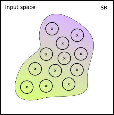
Formally, adversarial training uses projected gradient descent to maximise the loss over the ball, projecting any perturbation that escapes the ball back inside, and then minimises the result over the network’s parameters. The objective, due to Madry et al. (2017) Madry, A., Makelov, A., Schmidt, L., Tsipras, D., & Vladu, A. (2017). Towards deep learning models resistant to adversarial attacks. arXiv Preprint arXiv:1706.06083. , is:

The inner maximisation finds the perturbation within of the data point that produces the largest loss; the outer minimisation finds the parameters that make that worst-case loss as small as possible.

What adversarial training actually optimises

Adversarial training works, and for -ball robustness on image classifiers it is the standard answer. But it is worth being precise about which property it improves, because the answer is narrower than it first appears — and this is where Part II begins.

Recall how Chapter 3 stated robustness: . That leaves undefined, and different ways of filling it in give genuinely different properties. Casadio et al. (2022) Casadio, M., Komendantskaya, E., Daggitt, M. L., Kokke, W., Katz, G., Amir, G., & Refaeli, I. (2022). Neural Network Robustness as a Verification Property: A Principled Case Study. Computer Aided Verification - 34th International Conference, CAV 2022, Haifa, Israel, August 7-10, 2022, Proceedings, Part I, 13371, 219–231. set them side by side:

DL2 training refers to the method of Fischer et al. (2019) Fischer, M., Balunovic, M., Drachsler-Cohen, D., Gehr, T., Zhang, C., & Vechev, M. T. (2019). DL2: Training and Querying Neural Networks with Logic. Proceedings of the 36th International Conference on Machine Learning, ICML 2019, 9-15 June 2019, Long Beach, California, USA, 97, 1931–1941. http://proceedings.mlr.press/v97/fischer19a.html ; is the confidence margin it requires of the advised class.

Projected gradient descent optimises exactly one row of this table: it minimises how far the output can move within the ball, which is standard robustness. Chapter 3’s specification, meanwhile, asks that the advised label stays the same, which is classification robustness — a different row.

The two are not in an implication relation in either direction. So it is entirely possible, and in the literature common, to train for one property, verify another, and report the result as though a single notion of robustness had been improved. Getting more of what you optimised while gaining nothing you verified is not a subtle failure mode; it is the expected outcome of a mismatch nobody wrote down.

This is the first of three difficulties that motivate the rest of the chapter.

Part II — Property-driven training

Part I ended on a mismatch: adversarial training optimises standard robustness while our specification asks for classification robustness. That is one instance of a general problem. The machine-learning toolkit was built for one property, on one kind of input region, in one application domain; a specification language lets us write down far more than that. This is the third of the challenges listed in Chapter 1, integrating property-driven training with verification. This part follows the framework of Flinkow et al. (Flinkow et al., 2025) Flinkow, T., Casadio, M., Kessler, C., Monahan, R., & Komendantskaya, E. (2025). A General Framework for Property-Driven Machine Learning. , which sets out what has to change, and why Vehicle is organised the way it is.

Three difficulties stand between the standard recipe and training for arbitrary specifications. We take them in turn.

Problem 1: specifications and objectives come apart

The table at the end of Part I is the first difficulty in miniature. Turning a logical specification into an optimisation objective is done by hand, and when it goes wrong nothing complains: training proceeds, the loss falls, and the verifier reports no improvement, because the quantity minimised was never the quantity checked. Casadio et al. (2022) Casadio, M., Komendantskaya, E., Daggitt, M. L., Kokke, W., Katz, G., Amir, G., & Refaeli, I. (2022). Neural Network Robustness as a Verification Property: A Principled Case Study. Computer Aided Verification - 34th International Conference, CAV 2022, Haifa, Israel, August 7-10, 2022, Proceedings, Part I, 13371, 219–231. draw the consequence: one kind of robustness does not imply another, so optimising for one can achieve very little for another. What is needed is not a better hand-translation but a systematic one, a single source from which both the verification query and the training objective are derived. That is what a specification language can provide, and it is why training belongs inside the verification toolchain rather than beside it.

Problem 2: from -balls to hyper-rectangles

The second difficulty is the shape of the input region. Adversarial training assumes an -norm ball around a data point,

which suits images, where a small perturbation of every pixel is a meaningful notion of “nearby”. It suits other domains badly.

In natural language processing the input space is discrete, and an -ball around a sentence contains no sentences; the region that matters is the set of semantically similar sentences, which is not a ball around anything. In the cyber-physical systems of Chapter 2 the input space is low-dimensional and the interesting regions are named by the specification itself: “intruder directly ahead and moving towards us” is a constraint on five variables with different units and ranges, not a ball.

The generalisation is to a hyper-rectangle, an independent interval per dimension:

Any conjunction of bounds on individual inputs describes one. Recall this constraint from Chapter 2:

directlyAhead : UnnormalisedInput -> Bool
directlyAhead x =
  1500  <= x ! distanceToIntruder <= 1800 and
  -0.06 <= x ! angleToIntruder    <= 0.06

movingTowards : UnnormalisedInput -> Bool
movingTowards x =
  x ! intruderHeading >= 3.10  and
  x ! speed           >= 980   and
  x ! intruderSpeed   >= 960

These constraints give rise to the following hyper-rectangle in five-dimensional space:

The upper bounds for , and are the maximum input values from the ACAS Xu specification in Chapter 2. Every -ball is a hyper-rectangle with and , so nothing is lost, and regions that no ball can express become available. The training objective generalises by substitution: where adversarial training maximises over , we maximise over .

Problem 3: beyond “classify this as ”

The third difficulty is on the output side. Classification robustness assumes the goal is to keep the predicted class fixed. Many specifications say something less prescriptive.

ACAS Xu’s third property, which Chapter 2 verified, asks that if the intruder is directly ahead and closing, then the score for clear-of-conflict will not be minimal. It does not say which advisory the network should give — only that one of the four alternatives must outrank one particular option. Written out, the conclusion is a disjunction:

There is no label to hold fixed here, so there is nothing for the standard recipe to maximise. What is needed is a way to take an arbitrary specification and produce a differentiable loss that measures how far the network is from satisfying it. Such translations are called differentiable logics.

Differentiable logics

A differentiable logic replaces the Boolean connectives with real-valued, differentiable ones, so that a formula evaluates to a number that can be minimised rather than a truth value that cannot. A very small example over a toy language conveys the idea:

An atom is translated into the margin by which it holds or fails, and the connectives combine margins. Several such logics exist, and they differ in ways that matter for optimisation ( Fischer et al., 2019; Slusarz et al., 2023; van Krieken et al., 2022) Fischer, M., Balunovic, M., Drachsler-Cohen, D., Gehr, T., Zhang, C., & Vechev, M. T. (2019). DL2: Training and Querying Neural Networks with Logic. Proceedings of the 36th International Conference on Machine Learning, ICML 2019, 9-15 June 2019, Long Beach, California, USA, 97, 1931–1941. http://proceedings.mlr.press/v97/fischer19a.html Slusarz, N., Komendantskaya, E., Daggitt, M. L., Stewart, R. J., & Stark, K. (2023). Logic of Differentiable Logics: Towards a Uniform Semantics of DL. LPAR 2023: Proceedings of 24th International Conference on Logic for Programming, Artificial Intelligence and Reasoning, Manizales, Colombia, 4-9th June 2023, 94, 473–493. van Krieken, E., Acar, E., & van Harmelen, F. (2022). Analyzing Differentiable Fuzzy Logic Operators. Artif. Intell., 302, 103602. . The logic we adopt is quantitative linear logic (QLL), due to Capucci et al. (2026) Capucci, M., Atkey, R., Grellois, C., & Komendantskaya, E. (2026). Quantitative Linear Logic. :

Negation:

Conjunction:

Disjunction:

Implication:

where is the hardness degree. As the connectives converge on and , their traditional counterparts; smaller gives a smoother surface whose gradients reach further. Conjunction and disjunction are the familiar log-sum-exp softening of and , which is what makes them differentiable everywhere.

Note that the truth direction is reversed: is the top and is the bottom. This is usual in the differentiable logic literature, DL2 (Fischer et al., 2019) Fischer, M., Balunovic, M., Drachsler-Cohen, D., Gehr, T., Zhang, C., & Vechev, M. T. (2019). DL2: Training and Querying Neural Networks with Logic. Proceedings of the 36th International Conference on Machine Learning, ICML 2019, 9-15 June 2019, Long Beach, California, USA, 97, 1931–1941. http://proceedings.mlr.press/v97/fischer19a.html included, because the value measures how far a formula is from being satisfied — the less error there is, the more true the formula is. It also means that a loss built this way is unbounded below, which matters when it is combined with a task loss.

The property-driven objective

The three pieces now assemble. Standard training minimises the expected task loss over the data:

Adversarial training minimises it against the worst case in an -ball, and Problem 2 replaces that ball with a hyper-rectangle:

Problem 3 adds the specification itself as a second term, translated by the differentiable logic, and balances the two:

This single objective has the earlier methods as special cases. Setting recovers adversarial training over a general region. Taking to be the -cube around and to be recovers standard robustness — the row of Part I’s table that adversarial training optimises. And a specification with no input constraint at all, , is handled by letting be the domain of the input, typically the normalisation bounds , .

Both extremes of are worth understanding. At the specification is ignored. At the task is ignored, and since a constant network satisfies most robustness properties perfectly, the optimiser is free to discard the classifier altogether — the constraint term alone does not distinguish a useful constant from a useless one. The blend is not a convenience; it is what rules out the degenerate solution. Exercise #6 shows what this looks like when is forced by the absence of data, and what can stand in for the blend.

Property-driven training in Vehicle

Vehicle’s answer to Problem 1 is to derive both artefacts from one source. The same .vcl specification that Chapter 3 compiled into verification queries can be compiled into a loss function, so the property being trained for and the property being verified are the same text. Nothing is hand-translated, and the two cannot drift apart.

The interface mirrors the objective above. load_specification takes the specification and a differentiable logic and returns the named properties, each as a callable that evaluates for a batch; alpha in the training loop is the of the objective, balancing task loss against constraint loss.

Vehicle has two built-in logics, VehicleDifferentiableLogic and DL2DifferentiableLogic; the code below selects the first. The Capucci logic of the previous section can be declared directly in the specification as a DifferentiableTensorLogic and selected by name with vcl.CustomDifferentiableLogic("qllAdditive"), which is what the experiment at the end of the chapter does.

Next, we will load our Vehicle specification and define our constraint loss function:

import vehicle_lang as vcl
from vehicle_lang.loss import pytorch as loss_pt

spec = loss_pt.load_specification(
    "fmnist-robustness.vcl",
    logic=vcl.VehicleDifferentiableLogic(),
)

constraint_loss_fn = spec["robust"]

import vehicle_lang as vcl
from vehicle_lang.loss import tensorflow as loss_tf

spec = loss_tf.load_specification(
    "fmnist-robustness.vcl",
    logic=vcl.VehicleDifferentiableLogic(),
)

constraint_loss_fn = spec["robust"]

The first parameter to the load_specification function is the path to the Vehicle specification. The second parameter defines which logic to use; it is optional, and defaults to DL2DifferentiableLogic. We define which property from the specification to use as our constraint loss function by accessing it by name on the specification object.

Next, we will define a simple model and training procedure. This is the minimal version of the loop, at and alpha = 0.5 with the built-in logic; the experiment at the end of the chapter changes those three settings, for reasons Part I has already given, and otherwise runs exactly this code.

import torch
import torch.nn as nn

model = nn.Sequential(
    nn.Flatten(),
    nn.Linear(784, 64),
    nn.ReLU(),
    nn.Linear(64, 32),
    nn.ReLU(),
    nn.Linear(32, 10)
)

def network(x: torch.Tensor) -> torch.Tensor:
    return model(x.reshape(1, 1, 28, 28)).reshape(10)

optimizer = torch.optim.Adam(model.parameters(), lr=1e-3)
cross_entropy = nn.CrossEntropyLoss()

num_epochs = 5
alpha = 0.5

for epoch in range(num_epochs):
    for step, (images, labels) in enumerate(train_loader):
        optimizer.zero_grad()
        logits = model(images)
        loss = cross_entropy(logits, labels)

        constraint_loss = constraint_loss_fn(
            n=BATCH_SIZE,
            classifier=network,
            epsilon=torch.tensor(0.005),
            trainingImages=images.squeeze(1),
            trainingLabels=labels
        )

        constraint_loss = torch.stack(constraint_loss).mean()
        total_loss = alpha * loss + (1 - alpha) * constraint_loss

        total_loss.backward()
        optimizer.step()

from tensorflow.keras import layers, Sequential

model = Sequential([
    layers.InputLayer(shape=(1, 28, 28)),
    layers.Flatten(),
    layers.Dense(64, activation="relu"),
    layers.Dense(32, activation="relu"),
    layers.Dense(10)
])

def network(x: tf.Tensor) -> tf.Tensor:
    return tf.reshape(model(tf.reshape(x, (1, 1, 28, 28))), (10,))

optimizer = tf.keras.optimizers.Adam(learning_rate=1e-3)
cross_entropy = tf.keras.losses.SparseCategoricalCrossentropy(from_logits=True)

num_epochs = 5
alpha = 0.5

for epoch in range(num_epochs):
    for step, (images, labels) in enumerate(train_loader):
        with tf.GradientTape() as tape:
            logits = model(images)
            task_loss = cross_entropy(labels, logits)

            constraint_loss = constraint_loss_fn(
                n=BATCH_SIZE,
                classifier=network,
                epsilon=tf.constant(0.005),
                trainingImages=tf.squeeze(images, axis=-1),
                trainingLabels=labels
            )

            constraint_loss = tf.reduce_mean(tf.stack(constraint_loss))
            total_loss = alpha * task_loss + (1 - alpha) * constraint_loss

        grads = tape.gradient(total_loss, model.trainable_variables)
        optimizer.apply_gradients(zip(grads, model.trainable_variables))

Note that the network callable must match the type of the network declared in the Vehicle specification. The alpha parameter can be used to tweak the weighting of task loss vs. constraint loss, which are blended together in total_loss.

The n=BATCH_SIZE argument is the reason SUBSET_SIZE had to divide evenly by BATCH_SIZE. The specification declares its data set size as an inferred parameter, n, and here each batch plays the role of the data set, so n must be exactly the number of images in the batch. Were the last batch of an epoch short, the value of n would no longer describe the images being passed alongside it. We can now export this trained model to verify it using Vehicle, with the hope that it is more robust as a result of training with constraint loss. Model exportation can be done like so:

import torch.onnx

model.eval()
input_tensor = torch.randn(1,1,28,28)

torch.onnx.export(
    model,
    input_tensor,
    "classifier.onnx", # file name
    external_data=False, # required for Marabou verification
)

model.export("classifier")

python -m tf2onnx.convert \
    --saved-model classifier \
    --output classifier.onnx

Does it work?

Part I left us with a network and a number. The network is the 100-epoch classifier trained on cross-entropy alone, at 99.5% training accuracy; the number is 22, the count of Chapter 3’s fifty test images it is provably robust on at , out of the 38 it classifies correctly. We also saw that training it further on cross-entropy pushes that number down. The question this chapter has been building towards is whether putting the specification into the objective pushes it back up, and whether it does so without sacrificing the classifier.

The cleanest way to answer that is to change nothing else. So the experiment takes that same network, loads its weights, and trains it for ten more epochs on the objective of the previous section, with the constraint loss compiled from the robustness specification. Every epoch’s network is exported and verified with Chapter 3’s command, unchanged, so each result lands directly beside the 22.

The experiment: specification and logic

The training specification is Chapter 3’s, with two changes. The first is that advises is stated non-strictly, classifier image ! label >= classifier image ! j for all j, because the loss compiler does not handle the j != label guard of the strict form: it compiles without complaint to a loss that is identically zero, so a network trained on the guarded form simply does not move (Exercise #6 meets the same guard in the ACAS Xu specification). The two differ only when the advised label ties with another, and on this problem they return identical verdicts for every image, so training on the non-strict property and verifying on the strict one is a like-for-like comparison.

The second is that the specification declares the differentiable logic it should be compiled with. Rather than the built-in default, we use the quantitative linear logic of Capucci et al. (2026) Capucci, M., Atkey, R., Grellois, C., & Komendantskaya, E. (2026). Quantitative Linear Logic. introduced in Part II, written out in Vehicle as a DifferentiableTensorLogic:

p : Real
p = 2.0

qllAdditive : DifferentiableTensorLogic
qllAdditive =
  { trueElement                = -infinity
  , falseElement               = infinity
  , pointwiseNegation          = \x -> -x
  , pointwiseConjunction       = \{dims} x y -> (const (1/p) dims) * log(exp(const p dims * x) + exp(const p dims * y))
  , pointwiseDisjunction       = \{dims} x y -> -(const (1/p) dims) * log(exp(const (-p) dims * x) + exp(const (-p) dims * y))
  , pointwiseLessThan          = \x y -> x - y
  , pointwiseLessEqualThan     = \x y -> x - y
  , pointwiseGreaterThan       = \x y -> y - x
  , pointwiseGreaterEqualThan  = \x y -> y - x
  , pointwiseEqual             = \x y -> max (x - y) (y - x)
  , pointwiseNotEqual          = \x y -> - max (x - y) (y - x)
  , reduceConjunction          = \{dims} xs -> (1/p) * log(reduceAdd (exp (const p dims * xs)))
  , reduceDisjunction          = \{dims} xs -> (1/p) * log(reduceAdd (exp (const (-p) dims * xs)))
  }

Each line is one of the definitions from the section on differentiable logics: negation is , conjunction and disjunction are the log-sum-exp softenings of and with hardness , and a comparison becomes the margin by which it holds, so that compiles to , which is at most zero when true. The reduce forms are the same connectives applied across a tensor, which is how forall j over the ten labels is handled. Selecting it on the Python side is one argument:

spec = loss_pt.load_specification(
    "fashionRobustness-capucci.vcl",
    logic=vcl.CustomDifferentiableLogic("qllAdditive"),
)
constraint_loss_fn = spec["robust"]

One consequence of the definitions is worth noticing before training, because it explains the numbers that follow. advises quantifies over every label, including the advised one, and for that label the margin y - x is exactly zero. The soft maximum of a set of margins one of which is zero is at least zero. So the compiled loss for an image is zero when the whole neighbourhood is classified correctly, and positive otherwise; it exerts a force only on the images that are breakable. The task loss holds the classification in place while that force acts.

The experiment: the run

The settings are those of the previous section with two changes, both of which Part I argued for: rather than , because leaves one image to win back and leaves sixteen, and , so the constraint term carries slightly more weight than the task term. Otherwise: the same 1024 training images in batches of 64, Adam at , ten epochs, no clamping of the loss and no gradient clipping. On a CPU an epoch takes ten to fourteen minutes, because the constraint loss runs an adversarial search for every image in every batch; verifying fifty images takes between twelve and forty minutes per network and about 14 GB of memory.

The first three columns are measured during training, on the 1024 training images; the last three by Vehicle afterwards, on the fifty held-out test images, exactly as in Part I’s table. No image errored; one query timed out, on the epoch-2 network, and is counted as unverified.

What the experiment shows

Property-driven training gained provable robustness, on every snapshot. The starting network proves 22 of the fifty images. All ten snapshots prove between 24 and 27, and the final one proves 27. As a share of the images each network classifies correctly, the only images that could possibly be proved, the baseline’s 57.9% became 61.5% to 73.0%.

It cost no accuracy. The number of test images classified correctly never fell below 37 and finished at 40, two above the starting network; cross-entropy stayed between 0.052 and 0.063 throughout, against 0.041 at the start. The final network is better than the starting one on both axes at once. Part I showed that cross-entropy alone erodes robustness once the data is fitted. The constraint term reverses that, and the task term did not have to give anything up for it. That is the blend of the previous section doing what it was designed to do.

Two things are worth knowing beyond the headline.

• The verified count plateaus after epoch 1 while the loss keeps falling. The ten counts were 27, 24, 26, 24, 25, 25, 25, 26, 27, 27. The loss is measured on the 1024 training images through an FGSM search, and the verification is exact on 50 held-out images, so later loss improvement is partly fitting rather than generalising, and partly tightening margins on perturbations the search can find but Marabou is not limited to.
• Consecutive snapshots differ by up to three images with no change in the objective. Twenty images are proved by all ten snapshots, sixteen by none, and fourteen flip. So a single snapshot carries an error bar of about plus or minus two on this test set. The evidence for the gain is that all ten sit above 22, not any one of them.

The same comparison can be made from scratch, with the two chapter scripts as they ship: vanilla_classifier.py and pt_classifier.py differ only in the constraint term, and each trains for five epochs. Their networks classify 33 and 34 of the fifty images correctly, so the ceilings match; at the plain one proves 25 and the property-driven one 29, and at , the radius the constraint was trained at, 30 against 32. The margin is smaller, as it should be after five epochs at a radius where there is little to win, and the plain run is unseeded, so read it as consistent with the table above rather than as a second proof of it.

Where this leaves us

Part II set out three problems. The experiment answers the first directly: the property that was trained for and the property that was verified are the same .vcl text, compiled two ways, and nothing was translated by hand. It does not exercise the other two, since its input region is an -cube and its conclusion holds one label fixed. That said, this chapter has already set up everything you need to handle more complex specifications. Exercises #6 and #7 below explain what experiments to run to see Vehicle in action on Problems 2 and 3.

Chapter 6 will return to specifications of this kind, and will show how the richer, real-life specifications described in Problems 2 and 3 arise naturally in the modelling of cyber-physical systems, where input regions are given by physical ranges and conclusions are bounds on what a controller may do rather than labels. Vehicle will be indispensable then, and the machinery is the same one this chapter has just shown at work: the same load_specification, the same blended objective, the same verification command.

Exercises

We will use symbols (⭑), (⭑⭑) and (⭑⭑⭑) to rate exercise difficulty: easy, moderate and hard.

Exercise #1 (⭑): Run the Chapter code

Download the required materials (or produce them yourself) and repeat the steps described in this chapter. All code used in this chapter is available from the tutorial repository.

Exercise #2 (⭑): Verifying and comparing networks

Use a Vehicle specification (either the one provided, or your own) to verify a property (e.g., robustness) of a network trained with a logical loss function, and compare this to one trained without a logical loss function. Which is more robust, which has the better task accuracy, and why?

Exercise #3 (⭑⭑): Further experimentation

Try various combinations of task loss functions, constraint loss functions, and alpha values. How do these affect each other? Is there a combination that makes the network more robust? Is there a combination that makes the network more accurate? What happens when you use multiple constraint loss functions simultaneously?

Exercise #4 (⭑⭑): Normalisation inside the network

Part I kept the pixels in and warned against normalising them. Rebuild the training-verification pipeline with normalisation, but placed inside the network as its first layer, so that the inputs the specification and the verifier see are still raw pixels. Train, export, and verify. What does Marabou say about the exported network, and why? Fix it by folding the normalisation into the first linear layer before exporting, check that the folded network computes the same function as the trained one, and verify again. The chapter code’s pt_classifier.py contains one solution.

Exercise #5 (⭑⭑⭑): Training a model from scratch

Finally, try creating your own model from scratch and repeat the experiments and comparisons described above. Explore the relationship between how complex a model is and to what degree it can satisfy robustness, and the effect robustness training can have on this.

Hint: a simple model is worse at spotting the difference between two different images. Does this make it more or less likely to be robust?

Exercise #6 (⭑⭑): The ACAS Xu benchmark

This is the first exercise about properties more complex than -ball robustness. In Chapter 2 you verified the ten ACAS Xu properties on the networks , and and found that most of them fail: , for instance, satisfies only Properties 1, 2 and 10, Properties 3, 4, 5 and 9 are falsified in seconds, and Properties 6, 7 and 8 are too hard for Marabou to decide within fifteen minutes. Using the property-driven training of this chapter, re-train one of these networks and see whether more properties become verifiable.

Two things make this harder than Fashion MNIST. There is no data set, so there is no task loss to hold the network to its job (), and with a single property that is fatal: training on Property 3 alone makes the property hold after one epoch by producing a network that never advises clear-of-conflict anywhere: the degenerate solution the objective section warned about, with no task term to rule it out. And the properties are stated with a guarded implication i != j => ... that the loss compiler turns into a constant loss, so the training specification must state minimalScore non-strictly without the guard, as fmnist-robustness.vcl does for the same reason.

Hint: split the specification into ten one-property files and train on them one property per epoch, repeatedly, so that the properties counterbalance each other and no single one gets to reshape the whole network; start a fresh optimiser each epoch, or the second visit to a property will diverge. Properties 6, 7 and 8 quantify over (almost) the whole input space, so Marabou has to case-split over most of the network’s 300 ReLUs; give them a time cap and do not expect a verdict. The starting material is in chapter-4/exercises/acas2 and a complete worked solution, which takes from three verified properties to six while keeping 90% of its original advisories, in chapter-4/solutions/acas2.

These are the verdicts you should have obtained in Chapter 2’s exercises, for the three shipped networks on the ten properties, with a 15-minute cap per property (✓ verified, ✗ falsified, t/o = undecided within the cap):

Note that some properties remain unverified for all three networks: Properties 3, 4, 5 and 9 are falsified on every one, 6 and 7 are undecided on every one, and 8 is falsified on one network and undecided on the other two. This may suggest that these properties are difficult or impossible to infer from data: the networks were trained on a data set sampled from a controller, and a property that no network has picked up from the data is a property the data does not exhibit clearly enough, or a property the network architecture cannot represent, which property-driven training may be able to supply.

Exercise #7 (⭑⭑⭑): Training for properties more complex than -ball robustness: the Iris data set

Recall the code and Vehicle specifications from Chapter 2, Exercise #4 (verification of a model trained on the Iris data set). For any of your properties that Marabou falsified, run property-driven training, and measure whether they become verifiable as a result. You may need to take into consideration the heuristics you learnt in this chapter, concerning the choice of parameters such as and , as well as data and model normalisation.

Hint: this exercise is only possible because Vehicle implements a more general property-driven procedure than (-ball) adversarial training.